Graphics.Dynamic.Plot.R2

Display

Static

plotPrerender :: ViewportConfig -> [DynamicPlottable] -> IO PlainGraphicsR2

Render a single view of a collection of plottable objects. This can be used the same way as plotWindow, but does not open any GTK but gives the result as-is.

If the objects contain animations, only the initial frame will be rendered.

Interactive

plotWindow :: [DynamicPlottable] -> IO GraphWindowSpec

Plot some plot objects to a new interactive GTK window. Useful for a quick preview of some unknown data or real-valued functions; things like selection of reasonable view range and colourisation are automatically chosen.

Example:

The individual objects you want to plot can be evaluated in multiple threads, so a single hard calculatation won't freeze the responsitivity of the whole window. Invoke e.g. from ghci +RTS -N4 to benefit from this.

ATTENTION: the window may sometimes freeze, especially when displaying complicated functions with fnPlot from ghci. This is apparently a kind of deadlock problem with one of the C libraries that are invoked, At the moment, we can recommend no better solution than to abort and restart ghci (or what else you use – iHaskell kernel, process, ...) if this occurs.

plotWindow' :: ViewportConfig -> [DynamicPlottable] -> IO GraphWindowSpec

Like plotWindow, but with explicit specification how the window is supposed to show up. (plotWindow uses the default configuration, i.e. def.)

Plottable objects

Class

class Plottable p where

Class for types that can be plotted in some canonical, “obvious” way. If you want to display something and don't know about any specific caveats, try just using plot!

Minimal complete definition

plot

Methods

plot :: p -> DynamicPlottable

Instances

Plottable DynamicPlottable

Methods

plot :: DynamicPlottable -> DynamicPlottable

Plottable p => Plottable [p]

Methods

plot :: [p] -> DynamicPlottable

Plottable p => Plottable (Maybe p)

Methods

plot :: Maybe p -> DynamicPlottable

Plottable p => Plottable (Option p)

Methods

plot :: Option p -> DynamicPlottable

Plottable (Shade ℝ²)

Methods

plot :: Shade ℝ² -> DynamicPlottable

Plottable (ConvexSet ℝ²)

Methods

plot :: ConvexSet ℝ² -> DynamicPlottable

Plottable (Shade' ℝ²)

Methods

plot :: Shade' ℝ² -> DynamicPlottable

Plottable (Cutplane (ℝ, ℝ))

Methods

plot :: Cutplane (ℝ, ℝ) -> DynamicPlottable

Plottable (Cutplane ℝ²)

Methods

plot :: Cutplane ℝ² -> DynamicPlottable

Plottable p => Plottable (MousePressed -> p)

Methods

plot :: (MousePressed -> p) -> DynamicPlottable

Plottable p => Plottable (MousePress -> p)

Methods

plot :: (MousePress -> p) -> DynamicPlottable

Plottable p => Plottable (MouseClicks -> p)

Methods

plot :: (MouseClicks -> p) -> DynamicPlottable

Plottable p => Plottable (ViewHeight -> p)

Methods

plot :: (ViewHeight -> p) -> DynamicPlottable

Plottable p => Plottable (ViewWidth -> p)

Methods

plot :: (ViewWidth -> p) -> DynamicPlottable

Plottable p => Plottable (ViewYCenter -> p)

Methods

plot :: (ViewYCenter -> p) -> DynamicPlottable

Plottable p => Plottable (ViewXCenter -> p)

Methods

plot :: (ViewXCenter -> p) -> DynamicPlottable

Plottable (PointsWeb (ℝ, ℝ) (Colour ℝ))

Methods

plot :: PointsWeb (ℝ, ℝ) (Colour ℝ) -> DynamicPlottable

Plottable (PointsWeb (ℝ, ℝ) (Shade (Colour ℝ)))

Methods

plot :: PointsWeb (ℝ, ℝ) (Shade (Colour ℝ)) -> DynamicPlottable

Plottable (PointsWeb ℝ² (Colour ℝ))

Methods

plot :: PointsWeb ℝ² (Colour ℝ) -> DynamicPlottable

Plottable (PointsWeb ℝ² (Shade (Colour ℝ)))

Methods

plot :: PointsWeb ℝ² (Shade (Colour ℝ)) -> DynamicPlottable

Plottable (PointsWeb ℝ (Shade' ℝ))

Methods

plot :: PointsWeb ℝ (Shade' ℝ) -> DynamicPlottable

Plottable (Shaded ℝ ℝ)

Methods

plot :: Shaded ℝ ℝ -> DynamicPlottable

Simple function plots

fnPlot :: (forall m. Object (RWDiffable ℝ) m => AgentVal (-->) m ℝ -> AgentVal (-->) m ℝ) -> DynamicPlottable

Plot a continuous function in the usual way, taking arguments from the x-Coordinate and results to the y one. The signature looks more complicated than it is; think about it as requiring a polymorphic Floating function. Any simple expression like fnPlot (\x -> sin x / cos (sqrt x)) will work.

Under the hood this uses the category of region-wise differentiable functions, RWDiffable, to prove that no details are omitted (like small high-frequency bumps). Note that this can become difficult for contrived cases like cos(1/sin x) – while such functions will never come out with aliasing artifacts, they also may not come out quickly at all. (But for well-behaved functions, using the differentiable category actually tends to be more effective, because the algorithm immediately sees when it can describe an almost-linear region with only a few line segments.)

This function is equivalent to using plot on an RWDiffable arrow.

paramPlot :: (forall m. (WithField ℝ PseudoAffine m, SimpleSpace (Needle m)) => AgentVal (-->) m ℝ -> (AgentVal (-->) m ℝ, AgentVal (-->) m ℝ)) -> DynamicPlottable

Plot a continuous, “parametric function”, i.e. mapping the real line to a path in ℝ².

continFnPlot :: (Double -> Double) -> DynamicPlottable

Plot an (assumed continuous) function in the usual way. Since this uses functions of actual Double values, you have more liberty of defining functions with range-pattern-matching etc., which is at the moment not possible in the :--> category.

However, because Double can't really prove properties of a mathematical function, aliasing and similar problems are not taken into account. So it only works accurately when the function is locally linear on pixel scales (what most other plot programs just assume silently). In case of singularities, the naïve thing is done (extend as far as possible; vertical line at sign change), which again is common enough though not really right.

We'd like to recommend using fnPlot whenever possible, which automatically adjusts the resolution so the plot is guaranteed accurate (but it's not usable yet for a lot of real applications).

tracePlot :: [(Double, Double)] -> DynamicPlottable

Plot a sequence of points (x,y). The appearance of the plot will be automatically chosen to match resolution and point density: at low densities, each point will simply get displayed on its own. When the density goes so high you couldn't distinguish individual points anyway, we switch to a “trace view”, approximating the probability density function around a “local mean path”, which is rather more insightful (and much less obstructive/clunky) than a simple cloud of independent points.

In principle, this should be able to handle vast amounts of data (so you can, say, directly plot an audio file); at the moment the implementation isn't efficient enough and will get slow for more than some 100000 data points.

lineSegPlot :: [(Double, Double)] -> DynamicPlottable

Simply connect the points by straight line segments, in the given order. Beware that this will always slow down the performance when the list is large; there is no &201d; as in tracePlot.

linregressionPlot :: forall x m y. (SimpleSpace m, Scalar m ~ ℝ, y ~ ℝ, x ~ ℝ) => (x -> m +> y) -> [(x, Shade' y)] -> (Shade' m -> DynamicPlottable -> DynamicPlottable -> DynamicPlottable) -> DynamicPlottable

colourPaintPlot :: ((Double, Double) -> Maybe (Colour Double)) -> DynamicPlottable

Plot a function that assigns every point in view a colour value.

> plotWindow [colourPaintPlot $ (x,y) -> case (x^2+y^2, atan2 y x) of (r,φ) -> guard (sin (7*φ-2*r) > r) >> Just (Dia.blend (tanh r) Dia.red Dia.green), unitAspect ]

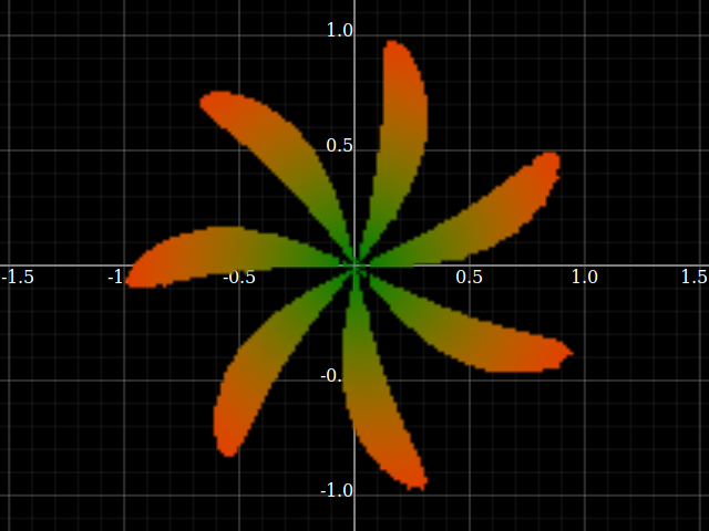
We try to evaluate that function no more often than necessary, but since it's a plain function with no differentiability information there's only so much that can be done; this requires a tradeoff between rasterisation fineness and performance. It works well for simple, smooth functions, but may not be adequate for functions with strong edges/transients, nor for expensive to compute functions.

type PlainGraphicsR2 = Diagram B

Use plot to directly include any Diagram. (All DynamicPlottable is internally rendered to that type.)

The exact type may change in the future: we'll probably stay with diagrams, but when document output is introduced the backend might become variable or something else but Cairo.

shapePlot :: PlainGraphicsR2 -> DynamicPlottable

Use a generic diagram within a plot.

Like with the various specialised function plotters, this will get automatically tinted to be distinguishable from other plot objects in the same window. Use diagramPlot instead, if you want to view the diagram as-is.

diagramPlot :: PlainGraphicsR2 -> DynamicPlottable

Plot a generic Diagram.

Multiple objects in one plot

plotMultiple :: Plottable x => [x] -> DynamicPlottable

Combine multiple objects in a single plot. Each will get an individual tint (if applicable). This is also the default behaviour of plotWindow.

To plot a family objects all with the same (but automatically-chosen) tint, simply use plot on the list, or combine them monoidally with <>.

Computation in progress

plotLatest :: Plottable x => [x] -> DynamicPlottable

Lazily consume the list, always plotting the latest value available as they arrive. Useful for displaying results of expensive computations that iteratively improve some result, but also for making simple animations (see plotDelay).

Plot-object attributes

Colour

tint :: Colour ℝ -> DynamicPlottable -> DynamicPlottable

Colour this plot object in a fixed shade.

autoTint :: DynamicPlottable -> DynamicPlottable

Allow the object to be automatically assigned a colour that's otherwise unused in the plot. (This is the default for most plot objects.)

Legend captions

legendName :: String -> DynamicPlottable -> DynamicPlottable

Set the caption for this plot object that should appear in the plot legend.

plotLegendPrerender :: LegendDisplayConfig -> [DynamicPlottable] -> IO (Maybe PlainGraphicsR2)

Render the legend (if any) belonging to a collection of plottable objects.

Animation

plotDelay :: NominalDiffTime -> DynamicPlottable -> DynamicPlottable

Limit the refresh / frame rate for this plot object. Useful to slowly study some sequence of plots with plotLatest, or to just reduce processor load.

Note: the argument will probably change to NominalDiffTime from the thyme library soon.

freezeAnim :: DynamicPlottable -> DynamicPlottable

Disable an animation, i.e. take an animated plot and show only the first frame.

startFrozen :: DynamicPlottable -> DynamicPlottable

Wait with starting the animation until the user has clicked on it.

Viewport

View selection

xInterval :: (Double, Double) -> DynamicPlottable

When you “plot” xInterval / yInterval, it is ensured that the (initial) view encompasses (at least) the specified range. Note there is nothing special about these “flag” objects: any Plottable can request a certain view, e.g. for a discrete point cloud it's obvious and a function defines at least a y-range for a given x-range. Only use explicit range when necessary.

yInterval :: (Double, Double) -> DynamicPlottable

forceXRange :: (Double, Double) -> DynamicPlottable

Like xInterval, this only affects what range is plotted. However, it doesn't merely request that a certain interval should be visible, but actually enforces particular values for the left and right boundary. Nothing outside the range will be plotted (unless there is another, contradicting forceXRange).

forceYRange :: (Double, Double) -> DynamicPlottable

unitAspect :: DynamicPlottable

Require that both coordinate axes are zoomed the same way, such that e.g. the unit circle will appear as an actual circle.

Interactive content

MouseClicks, ViewXCenter, ViewYResolution etc. can be used as arguments to some object you plot, if you want to plot stuff that depends on user interaction or just on the screen's visible range, for instance to calculate a tangent at the middle of the screen:

plotWindow [fnPlot sin, plot $ \(ViewXCenter xc) x -> sin xc + (x-xc) * cos xc]

newtype MousePressed

Constructors

MousePressed

Fields

• mouseIsPressedAt :: Maybe (ℝ, ℝ)

Instances

Plottable p => Plottable (MousePressed -> p)

Methods

plot :: (MousePressed -> p) -> DynamicPlottable

newtype MousePress

Constructors

MousePress

Fields

• lastMousePressedLocation :: (ℝ, ℝ)

Instances

Plottable p => Plottable (MousePress -> p)

Methods

plot :: (MousePress -> p) -> DynamicPlottable

newtype MouseClicks

Constructors

MouseClicks

Fields

• getClickPositions :: [(ℝ, ℝ)]

  A history of all clicks that were done in this window; more specifically, of all left mouse-button release events recorded.

Instances

Plottable p => Plottable (MouseClicks -> p)

Methods

plot :: (MouseClicks -> p) -> DynamicPlottable

clickThrough :: Plottable p => [p] -> DynamicPlottable

Move through a sequence of plottable objects, switching to the next whenever a click is received anywhere on the screen. Similar to plotLatest, but does not proceed automatically.

withDraggablePoints :: forall p list. (Plottable p, Traversable list) => list (ℝ, ℝ) -> (list (ℝ, ℝ) -> p) -> DynamicPlottable

Plot something dependent on points that the user can interactively move around. The nearest point (Euclidean distance) is always picked to be dragged.

mouseInteractive :: Plottable p => (MouseEvent (ℝ, ℝ) -> s -> s) -> s -> (s -> p) -> DynamicPlottable

data MouseEvent x

Instances

Eq x => Eq (MouseEvent x)

Methods

(==) :: MouseEvent x -> MouseEvent x -> Bool

(/=) :: MouseEvent x -> MouseEvent x -> Bool

clickLocation :: forall x. Lens' (MouseEvent x) x

releaseLocation :: forall x. Lens' (MouseEvent x) x

Displayed range

newtype ViewXCenter

Constructors

ViewXCenter

Fields

• getViewXCenter :: Double

Instances

Plottable p => Plottable (ViewXCenter -> p)

Methods

plot :: (ViewXCenter -> p) -> DynamicPlottable

newtype ViewYCenter

Constructors

ViewYCenter

Fields

• getViewYCenter :: Double

Instances

Plottable p => Plottable (ViewYCenter -> p)

Methods

plot :: (ViewYCenter -> p) -> DynamicPlottable

newtype ViewWidth

Constructors

ViewWidth

Fields

• getViewWidth :: Double

Instances

Plottable p => Plottable (ViewWidth -> p)

Methods

plot :: (ViewWidth -> p) -> DynamicPlottable

newtype ViewHeight

Constructors

ViewHeight

Fields

• getViewHeight :: Double

Instances

Plottable p => Plottable (ViewHeight -> p)

Methods

plot :: (ViewHeight -> p) -> DynamicPlottable

Resolution

newtype ViewXResolution

Constructors

ViewXResolution

Fields

• getViewXResolution :: Int

newtype ViewYResolution

Constructors

ViewYResolution

Fields

• getViewYResolution :: Int

Auxiliary plot objects

dynamicAxes :: DynamicPlottable

Coordinate axes with labels. For many plottable objects, these will be added automatically, by default (unless inhibited with noDynamicAxes).

noDynamicAxes :: DynamicPlottable

xAxisLabel :: String -> DynamicPlottable

yAxisLabel :: String -> DynamicPlottable

Types

The plot type

type DynamicPlottable = DynamicPlottable' RVar

tweakPrerendered :: (PlainGraphicsR2 -> PlainGraphicsR2) -> DynamicPlottable -> DynamicPlottable

Viewport choice

data ViewportConfig

Instances

Default ViewportConfig

Methods

def :: ViewportConfig

Resolution

xResV :: Lens' ViewportConfig Int

yResV :: Lens' ViewportConfig Int

Background

setSolidBackground :: Colour Double -> ViewportConfig -> ViewportConfig

Output scaling

prerenderScaling :: Lens' ViewportConfig PrerenderScaling

data PrerenderScaling

Constructors

ValuespaceScaling

The diagram has the original coordinates of the data that's plotted in it. E.g. if you've plotted an oscillation with amplitude 1e-4, the height of the plot will be indicated as only 0.0002. Mostly useful when you want to juxtapose multiple plots with correct scale matching.

NormalisedScaling

The diagram is scaled to have a range of [-1, 1] in both x- and y-direction.

OutputCoordsScaling

Scaled to pixel coordinates, i.e. the x range is [0, xResV-1] and the y range [0, yResV-1].

data LegendDisplayConfig

Instances

Default LegendDisplayConfig

Methods

def :: LegendDisplayConfig

legendPrerenderSize :: Iso' LegendDisplayConfig (SizeSpec V2 Double)

General

graphicsPostprocessing :: Lens' ViewportConfig (PlainGraphicsR2 -> PlainGraphicsR2)