Graphics.Rendering.Plot.Light

plot-light provides functionality for rendering vector graphics in SVG format. It is geared in particular towards scientific plotting, and it is termed "light" because it only requires a few common Haskell dependencies and no external libraries.

Usage

To incorporate this library in your projects you just need import Graphics.Rendering.Plot.Light. If GHC complains of name collisions you must import the module in "qualified" form.

Examples

If you wish to try out the examples in this page, you will need to have these import statements as well :

import Text.Blaze.Svg.Renderer.String (renderSvg) 
import qualified Data.Colour.Names as C
import qualified Data.Text.IO as T (readFile, writeFile)
import qualified Data.Text as T

1. Heatmap plot of a 2D function

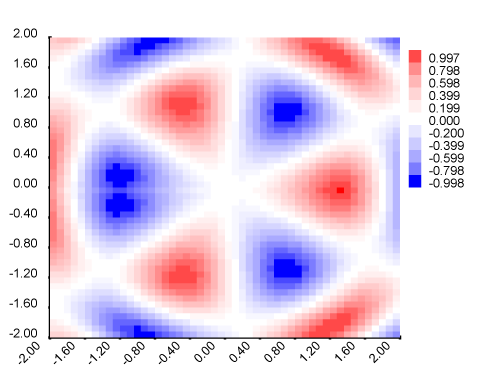
This example renders the function

\[ {f(x, y) = \cos(\pi \theta) \sin( \rho^2) } \] where \( \rho^2 = x^2 + y^2 \) and \( \theta = \arctan(y/x) \).

xPlot = 400
yPlot = 300

fdat = FigureData xPlot yPlot 0.1 0.8 0.1 0.9 10

palette0 = palette [C.red, C.white, C.blue] 15

plotFun2ex1 = do
 let 
   p1 = Point (-2) (-2)
   p2 = Point 2 2
   frame = mkFrame p1 p2
   nx = 50 
   ny = 50
   f x y = cos ( pi * theta ) * sin r 
     where
       r = x'**2 + y'**2
       theta = atan2 y' x'
       (x', y') = (fromRational x, fromRational y)
   lps = plotFun2 f $ meshGrid frame nx ny
   vmin = minimum $ _lplabel <$> lps
   vmax = maximum $ _lplabel <$> lps   
   pixels = heatmap' fdat palette0 frame nx ny lps
   cbar = colourBar fdat palette0 10 vmin vmax 10 TopRight 100
   svg_t = svgHeader xPlot yPlot $ do
      axes fdat frame 2 C.black 10 10
      pixels
      cbar
 T.writeFile "heatmap.svg" $ T.pack $ renderSvg svg_t

This example demonstrates how to plot a 2D scalar function and write the output to SVG file.

First, we define a FigureData object (which holds the SVG figure dimensions and parameters for the white margin around the rendering canvas) and a palette.

Afterwards we declare a Frame that bounds the rendering canvas using mkFrame. This is discretized in nx by ny pixels with meshGrid, and the function f is computed at the intersections of the mesh with plotFun2.

The axes function adds labeled axes to the figure; the user just needs to specify stroke width and color and how many ticks to display.

The data to be plotted (represented in this case as a list of LabeledPoints, in which the "label" carries the function value) are then mapped onto the given colour palette and drawn to the SVG canvas as a heatmap', i.e. a mesh of filled rectangles (Caution: do not exceed resolutions of ~ hundred pixels per side).

Next, we create the legend; in this case this is a colourBar element that requires the data bounds vmin, vmax.

As a last step, the SVG content is wrapped in the appropriate markdown by svgHeader and written to file.

2. Scatter plot of 3D data

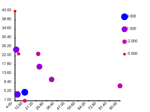
This example shows how to plot a collection of labelled points in the plane. Each sample row is represented by a LabeledPoint, in which the label is a scalar quantity.

The scatterLP function renders each data row as a glyph, by modifying a ScatterPointData record of default values via three functions that control the glyph size, contour line thickness and colour. This functionality can be exploited in creative ways to achieve effective infographics.

xPlot = 400
yPlot = 300
fnameOut = "data/scatter-1.svg"

fdat = FigureData xPlot yPlot 0.1 0.8 0.1 0.9 10

dats = zipWith LabeledPoint p_ l_ where
  l_ = [-5, -4 .. ]
  p_ = zipWith Point [4,7,12,23,90,34,24,5,6,12,3] [43,23,1,23,8,11,17,25,4,5]

spdata = ScatterPointData Circle 3 3 C.red


main = do
 let
   frameTo = frameFromFigData fdat
   frameFrom = frameFromPoints $ _lp <$> dats
   vmin = minimum $ _lplabel <$> dats
   vmax = maximum $ _lplabel <$> dats     
   f l sz = 10/(1 + exp(-(0.3 * x)))
     where x = l + sz
   g _ w = w
   h l col = C.blend l' C.blue col
     where
       l' = (l - vmin)/(vmax - vmin)
   dats' = moveLabeledPointBwFrames frameFrom frameTo False True <$> dats
   svg_t = svgHeader xPlot yPlot $ do
     axes fdat frameFrom 2 C.black 10 10
     scatterLP f g h spdata dats'
     scatterLPBar fdat 50 vmin vmax 3 TopRight 100 f g h spdata
  T.writeFile fnameOut $ T.pack $ renderSvg svg_t

Plot types

Heatmap

heatmap

Arguments

:: FigureData Rational

Figure data

-> [Colour Double]

Colour palette

-> [[Scientific]]

Data

-> Svg

heatmap assumes the input data corresponds to evenly sampled values of a scalar-valued field, and it maps the data values onto the provided palette (which can be created e.g. with brewerSet).

heatmap'

Arguments

:: (Foldable f, Functor f, Show a, RealFrac a, RealFrac t)

=> FigureData a

Figure data

-> [Colour Double]

Colour palette

-> Frame a

Frame containing the data

-> a

Number of points along x axis

-> a

" y axis

-> f (LabeledPoint t a)

Data

-> Svg

heatmap' renders one SVG pixel for every LabeledPoint supplied as input. The LabeledPoints must be bounded by the Frame.

plotFun2 :: Functor f => (t -> t -> l) -> f (Point t) -> f (LabeledPoint l t)

Plot a scalar function f of points in the plane (i.e. \(f : \mathbf{R}^2 \rightarrow \mathbf{R}\))

colourBar

Arguments

:: (RealFrac t, RealFrac a, Show a, Enum t, Floating a)

=> FigureData (Ratio Integer)

Figure data

-> [Colour Double]

Palette

-> a

Width

-> t

Value range minimum

-> t

Value range maximum

-> Int

Number of distinct values

-> LegendPosition_

Legend position in the figure

-> a

Colour bar length

-> Svg

A colour bar legend, to be used within heatmap-style plots.

Scatter

scatter :: (Foldable t, Show a, RealFrac a) => ScatterPointData a -> t (Point a) -> Svg

Scatter plot

Every point in the plot has the same parameters, as declared in the ScatterPointData record

scatterLP :: (Foldable t, RealFrac a, Show a) => (l -> b -> a) -> (l -> b -> a) -> (l -> Colour Double -> Colour Double) -> ScatterPointData b -> t (LabeledPoint l a) -> Svg

Parametric scatter plot

The parameters of every point in the scatter plot are modulated according to the label, using the three functions.

This can be used to produce rich infographics, in which e.g. the colour and size of the glyphs carry additional information.

scatterLPBar :: (RealFrac t, Enum t, RealFrac b, Show b) => FigureData b -> b -> t -> t -> Int -> LegendPosition_ -> b -> (t -> b -> b) -> (t -> b -> b) -> (t -> Colour Double -> Colour Double) -> ScatterPointData b -> Svg

data ScatterPointData a

Parameters for a scatterplot glyph

Constructors

ScatterPointData

Fields

• spGlyphShape :: GlyphShape_
• spSize :: a
• spStrokeWidth :: a
• spColour :: Colour Double

Instances

Eq a => Eq (ScatterPointData a)

Methods

(==) :: ScatterPointData a -> ScatterPointData a -> Bool

(/=) :: ScatterPointData a -> ScatterPointData a -> Bool

Show a => Show (ScatterPointData a)

Methods

showsPrec :: Int -> ScatterPointData a -> ShowS

show :: ScatterPointData a -> String

showList :: [ScatterPointData a] -> ShowS

data GlyphShape_

Glyph shape

Constructors

Square

Circle

Cross

Plus

Instances

Enum GlyphShape_

Methods

succ :: GlyphShape_ -> GlyphShape_

pred :: GlyphShape_ -> GlyphShape_

toEnum :: Int -> GlyphShape_

fromEnum :: GlyphShape_ -> Int

enumFrom :: GlyphShape_ -> [GlyphShape_]

enumFromThen :: GlyphShape_ -> GlyphShape_ -> [GlyphShape_]

enumFromTo :: GlyphShape_ -> GlyphShape_ -> [GlyphShape_]

enumFromThenTo :: GlyphShape_ -> GlyphShape_ -> GlyphShape_ -> [GlyphShape_]

Eq GlyphShape_

Methods

(==) :: GlyphShape_ -> GlyphShape_ -> Bool

(/=) :: GlyphShape_ -> GlyphShape_ -> Bool

Show GlyphShape_

Methods

showsPrec :: Int -> GlyphShape_ -> ShowS

show :: GlyphShape_ -> String

showList :: [GlyphShape_] -> ShowS

Plot elements

Geometrical primitives

rect

Arguments

:: (Show a, RealFrac a)

=> a

Width

-> a

Height

-> a

Stroke width

-> Maybe (Colour Double)

Stroke colour

-> Maybe (Colour Double)

Fill colour

-> Point a

Corner point coordinates

-> Svg

A rectangle, defined by its anchor point coordinates and side lengths

> putStrLn $ renderSvg $ rect (Point 100 200) 30 60 2 Nothing (Just C.aquamarine)
<rect x="100.0" y="200.0" width="30.0" height="60.0" fill="#7fffd4" stroke="none" stroke-width="2.0" />

rectCentered

Arguments

:: (Show a, RealFrac a)

=> a

Width

-> a

Height

-> a

Stroke width

-> Maybe (Colour Double)

Stroke colour

-> Maybe (Colour Double)

Fill colour

-> Point a

Center coordinates

-> Svg

A rectangle, defined by its center coordinates and side lengths

> putStrLn $ renderSvg $ rectCentered 15 30 1 (Just C.blue) (Just C.red) (Point 20 30)
<rect x="12.5" y="15.0" width="15.0" height="30.0" fill="#ff0000" stroke="#0000ff" stroke-width="1.0" />

squareCentered :: (Show a, RealFrac a) => a -> a -> Maybe (Colour Double) -> Maybe (Colour Double) -> Point a -> Svg

circle

Arguments

:: (Real a1, Real a)

=> a

Radius

-> a

Stroke width

-> Maybe (Colour Double)

Stroke colour

-> Maybe (Colour Double)

Fill colour

-> Point a1

Center

-> Svg

A circle

> putStrLn $ renderSvg $ circle (Point 20 30) 15 (Just C.blue) (Just C.red)
<circle cx="20.0" cy="30.0" r="15.0" fill="#ff0000" stroke="#0000ff" />

line

Arguments

:: (Show a, RealFrac a)

=> Point a

First point

-> Point a

Second point

-> a

Stroke width

-> LineStroke_ a

Stroke type

-> Colour Double

Stroke colour

-> Svg

Line segment between two Points

> putStrLn $ renderSvg $ line (Point 0 0) (Point 1 1) 0.1 Continuous C.blueviolet
<line x1="0.0" y1="0.0" x2="1.0" y2="1.0" stroke="#8a2be2" stroke-width="0.1" />

> putStrLn $ renderSvg (line (Point 0 0) (Point 1 1) 0.1 (Dashed [0.2, 0.3]) C.blueviolet)
<line x1="0.0" y1="0.0" x2="1.0" y2="1.0" stroke="#8a2be2" stroke-width="0.1" stroke-dasharray="0.2, 0.3" />

text

Arguments

:: (Show a, Real a)

=> a

Rotation angle of the textbox

-> Int

Font size

-> Colour Double

Font colour

-> TextAnchor_

How to anchor the text to the point

-> Text

Text

-> V2 a

Displacement w.r.t. rotated textbox

-> Point a

Initial position of the text box (i.e. before rotation and displacement)

-> Svg

text renders text onto the SVG canvas

Conventions

The Point argument p refers to the lower-left corner of the text box.

The text box can be rotated by rot degrees around p and then anchored at either its beginning, middle or end to p with the TextAnchor_ flag.

The user can supply an additional V2 displacement which will be applied after rotation and anchoring and refers to the rotated text box frame.

> putStrLn $ renderSvg $ text (-45) C.green TAEnd "blah" (V2 (- 10) 0) (Point 250 0)
<text x="-10.0" y="0.0" transform="translate(250.0 0.0)rotate(-45.0)" fill="#008000" text-anchor="end">blah</text>

polyline

Arguments

:: (Foldable t, Show a1, Show a, RealFrac a, RealFrac a1)

=> a1

Stroke width

-> LineStroke_ a

Stroke type

-> StrokeLineJoin_

Stroke join type

-> Colour Double

Stroke colour

-> t (Point a)

Data

-> Svg

Polyline (piecewise straight line)

> putStrLn $ renderSvg (polyline [Point 100 50, Point 120 20, Point 230 50] 4 (Dashed [3, 5]) Round C.blueviolet)
<polyline points="100.0,50.0 120.0,20.0 230.0,50.0" fill="none" stroke="#8a2be2" stroke-width="4.0" stroke-linejoin="round" stroke-dasharray="3.0, 5.0" />

filledPolyline

Arguments

:: (Foldable t, Show a, Real o)

=> Colour Double

Fill colour

-> o

Fill opacity

-> t (Point a)

Contour point coordinates

-> Svg

A filled polyline

> putStrLn $ renderSvg $ filledPolyline C.coral 0.3 [(Point 0 1), (Point 10 40), Point 34 50, Point 30 5]
<polyline points="0,1 10,40 34,50 30,5" fill="#ff7f50" fill-opacity="0.3" />

pixel :: (Show a, RealFrac a) => [Colour Double] -> a -> a -> Scientific -> Scientific -> LabeledPoint Scientific a -> Svg

pixel' :: (Show a, RealFrac a, RealFrac t) => [Colour Double] -> a -> a -> t -> t -> LabeledPoint t a -> Svg

Composite plot elements

filledBand

Arguments

:: (Foldable t, Real o, Show a)

=> Colour Double

Fill colour

-> o

Fill opacity

-> (l -> a)

Band maximum value

-> (l -> a)

Band minimum value

-> t (LabeledPoint l a)

Centerline points

-> Svg

A filled band of colour, given the coordinates of its center line

This element can be used to overlay uncertainty ranges (e.g. the first standard deviation) associated with a given data series.

candlestick

Arguments

:: (Show a, RealFrac a)

=> (a -> a -> Bool)

If True, fill the box with the first colour, otherwise with the second

-> (l -> a)

Box maximum value

-> (l -> a)

Box minimum value

-> (l -> a)

Line maximum value

-> (l -> a)

Line minimum value

-> a

Box width

-> a

Stroke width

-> Colour Double

First box colour

-> Colour Double

Second box colour

-> Colour Double

Line stroke colour

-> LabeledPoint l a

Data point

-> Svg

A candlestick glyph for time series plots. This is a type of box glyph, commonly used in plotting financial time series.

Some financial market quantities such as currency exchange rates are aggregated over some time period (e.g. a day) and summarized by various quantities, for example opening and closing rates, as well as maximum and minimum over the period.

By convention, the candlestick colour depends on the derivative sign of one such quantity (e.g. it is green if the market closes higher than it opened, and red otherwise).

Plot utilities

axes :: (Show a, RealFrac a) => FigureData a -> Frame a -> a -> Colour Double -> Int -> Int -> Svg

A pair of Cartesian axes

toPlot

Arguments

:: (Functor t, Foldable t, Show a, RealFrac a)

=> FigureData a

-> (l -> Text)

X tick label

-> (l -> Text)

Y tick label

-> a

X label rotation angle

-> a

Y label rotation angle

-> a

Stroke width

-> Colour Double

Stroke colour

-> Maybe (t (LabeledPoint l a))

X axis labels

-> Maybe (t (LabeledPoint l a))

Y axis labels

-> (t (LabeledPoint l a) -> Svg)

Data rendering function

-> t (LabeledPoint l a)

Data

-> Svg

toPlot performs a number of related operations:

• Maps the dataset to the figure frame
• Renders the X, Y axes
• Renders the transformed dataset onto the newly created plot canvas

data FigureData a

Figure data

Constructors

FigureData

Fields

• figWidth :: a

  Figure width

• figHeight :: a

  Figure height

• figLeftMFrac :: a

  Left margin fraction (w.r.t figure width)

• figRightMFrac :: a

  Right margin fraction (w.r.t figure width)

• figTopMFrac :: a

  Top margin fraction (w.r.t figure height)

• figBottomMFrac :: a

  Bottom margin fraction (w.r.t figure height)

• figLabelFontSize :: Int

  Tick label font size

Instances

Functor FigureData

Methods

fmap :: (a -> b) -> FigureData a -> FigureData b

(<$) :: a -> FigureData b -> FigureData a

Eq a => Eq (FigureData a)

Methods

(==) :: FigureData a -> FigureData a -> Bool

(/=) :: FigureData a -> FigureData a -> Bool

Show a => Show (FigureData a)

Methods

showsPrec :: Int -> FigureData a -> ShowS

show :: FigureData a -> String

showList :: [FigureData a] -> ShowS

Element attributes

data LineStroke_ a

Specify a continuous or dashed stroke

Constructors

Continuous

Dashed [a]

Instances

Eq a => Eq (LineStroke_ a)

Methods

(==) :: LineStroke_ a -> LineStroke_ a -> Bool

(/=) :: LineStroke_ a -> LineStroke_ a -> Bool

Show a => Show (LineStroke_ a)

Methods

showsPrec :: Int -> LineStroke_ a -> ShowS

show :: LineStroke_ a -> String

showList :: [LineStroke_ a] -> ShowS

data StrokeLineJoin_

Specify the type of connection between line segments

Constructors

Miter

Round

Bevel

Inherit

Instances

Eq StrokeLineJoin_

Methods

(==) :: StrokeLineJoin_ -> StrokeLineJoin_ -> Bool

(/=) :: StrokeLineJoin_ -> StrokeLineJoin_ -> Bool

Show StrokeLineJoin_

Methods

showsPrec :: Int -> StrokeLineJoin_ -> ShowS

show :: StrokeLineJoin_ -> String

showList :: [StrokeLineJoin_] -> ShowS

data TextAnchor_

Specify at which end should the text be anchored to its current point

Constructors

TAStart

TAMiddle

TAEnd

Instances

Eq TextAnchor_

Methods

(==) :: TextAnchor_ -> TextAnchor_ -> Bool

(/=) :: TextAnchor_ -> TextAnchor_ -> Bool

Show TextAnchor_

Methods

showsPrec :: Int -> TextAnchor_ -> ShowS

show :: TextAnchor_ -> String

showList :: [TextAnchor_] -> ShowS

data LegendPosition_

Constructors

TopLeft

TopRight

BottomLeft

BottomRight

Instances

Eq LegendPosition_

Methods

(==) :: LegendPosition_ -> LegendPosition_ -> Bool

(/=) :: LegendPosition_ -> LegendPosition_ -> Bool

Show LegendPosition_

Methods

showsPrec :: Int -> LegendPosition_ -> ShowS

show :: LegendPosition_ -> String

showList :: [LegendPosition_] -> ShowS

Colour utilities

blendTwo :: Colour Double -> Colour Double -> Int -> [Colour Double]

`blendTwo c1 c2 n` creates a palette of n intermediate colours, interpolated linearly between c1 and c2.

palette :: [Colour Double] -> Int -> [Colour Double]

`palette cs n` blends linearly a list of colours cs, by generating n intermediate colours between each consecutive pair.

pickColour :: RealFrac t => [Colour Double] -> t -> t -> t -> Colour Double

SVG utilities

svgHeader

Arguments

:: Real a

=> a

Image width (X axis)

-> a

Image height (Y axis)

-> Svg

Image content

-> Svg

Create the SVG header

translateSvg :: Show a => Point a -> Svg -> Svg

Move a Svg entity to a new position

Types

data Frame a

A frame, i.e. a bounding box for objects

Constructors

Frame

Fields

• _fpmin :: Point a
• _fpmax :: Point a

Instances

Eq a => Eq (Frame a)

Methods

(==) :: Frame a -> Frame a -> Bool

(/=) :: Frame a -> Frame a -> Bool

Show a => Show (Frame a)

Methods

showsPrec :: Int -> Frame a -> ShowS

show :: Frame a -> String

showList :: [Frame a] -> ShowS

(Ord a, Num a) => Monoid (Frame a)

The semigroup operation (mappend) applied on two Frames results in a new Frame that bounds both.

Methods

mempty :: Frame a

mappend :: Frame a -> Frame a -> Frame a

mconcat :: [Frame a] -> Frame a

data Point a

A Point object defines a point in the plane

Constructors

Point

Fields

• _px :: a
• _py :: a

Instances

Eq a => Eq (Point a)

Methods

(==) :: Point a -> Point a -> Bool

(/=) :: Point a -> Point a -> Bool

Show a => Show (Point a)

Methods

showsPrec :: Int -> Point a -> ShowS

show :: Point a -> String

showList :: [Point a] -> ShowS

data LabeledPoint l a

A LabeledPoint carries a "label" (i.e. any additional information such as a text tag, or any other data structure), in addition to position information. Data points on a plot are LabeledPoints.

Constructors

LabeledPoint

Fields

• _lp :: Point a

  The coordinates of the LabeledPoint (i.e. where in the figure it will be rendered)

• _lplabel :: l

  Data associated with the LabeledPoint

Instances

(Eq l, Eq a) => Eq (LabeledPoint l a)

Methods

(==) :: LabeledPoint l a -> LabeledPoint l a -> Bool

(/=) :: LabeledPoint l a -> LabeledPoint l a -> Bool

(Show l, Show a) => Show (LabeledPoint l a)

Methods

showsPrec :: Int -> LabeledPoint l a -> ShowS

show :: LabeledPoint l a -> String

showList :: [LabeledPoint l a] -> ShowS

labelPoint :: (Point a -> l) -> Point a -> LabeledPoint l a

Given a labelling function and a Point p, returned a LabeledPoint containing p and the computed label

mapLabel :: (l1 -> l2) -> LabeledPoint l1 a -> LabeledPoint l2 a

Apply a function to the label

data Axis

Constructors

X

Y

Instances

Eq Axis

Methods

(==) :: Axis -> Axis -> Bool

(/=) :: Axis -> Axis -> Bool

Show Axis

Methods

showsPrec :: Int -> Axis -> ShowS

show :: Axis -> String

showList :: [Axis] -> ShowS

Geometry

Vectors

data V2 a

V2 is a vector in R^2

Constructors

V2 a a

Instances

Eq a => Eq (V2 a)

Methods

(==) :: V2 a -> V2 a -> Bool

(/=) :: V2 a -> V2 a -> Bool

Show a => Show (V2 a)

Methods

showsPrec :: Int -> V2 a -> ShowS

show :: V2 a -> String

showList :: [V2 a] -> ShowS

Num a => Monoid (V2 a)

Vectors form a monoid w.r.t. vector addition

Methods

mempty :: V2 a

mappend :: V2 a -> V2 a -> V2 a

mconcat :: [V2 a] -> V2 a

Eps (V2 Double)

Methods

(~=) :: V2 Double -> V2 Double -> Bool

Eps (V2 Float)

Methods

(~=) :: V2 Float -> V2 Float -> Bool

Num a => Hermitian (V2 a)

Associated Types

type InnerProduct (V2 a) :: *

Methods

(<.>) :: V2 a -> V2 a -> InnerProduct (V2 a)

Num a => VectorSpace (V2 a)

Associated Types

type Scalar (V2 a) :: *

Methods

(.*) :: Scalar (V2 a) -> V2 a -> V2 a

Num a => AdditiveGroup (V2 a)

Vectors form an additive group

Methods

zero :: V2 a

(^+^) :: V2 a -> V2 a -> V2 a

(^-^) :: V2 a -> V2 a -> V2 a

Fractional a => MatrixGroup (DiagMat2 a) (V2 a)

Diagonal matrices can always be inverted

Methods

(<\>) :: DiagMat2 a -> V2 a -> V2 a

Num a => LinearMap (DiagMat2 a) (V2 a)

Methods

(#>) :: DiagMat2 a -> V2 a -> V2 a

Num a => LinearMap (Mat2 a) (V2 a)

Methods

(#>) :: Mat2 a -> V2 a -> V2 a

type InnerProduct (V2 a)

type InnerProduct (V2 a) = a

type Scalar (V2 a)

type Scalar (V2 a) = a

Matrices

data Mat2 a

A Mat2 can be seen as a linear operator that acts on points in the plane

Constructors

Mat2 a a a a

Instances

Eq a => Eq (Mat2 a)

Methods

(==) :: Mat2 a -> Mat2 a -> Bool

(/=) :: Mat2 a -> Mat2 a -> Bool

Show a => Show (Mat2 a)

Methods

showsPrec :: Int -> Mat2 a -> ShowS

show :: Mat2 a -> String

showList :: [Mat2 a] -> ShowS

Num a => Monoid (Mat2 a)

Matrices form a monoid w.r.t. matrix multiplication and have the identity matrix as neutral element

Methods

mempty :: Mat2 a

mappend :: Mat2 a -> Mat2 a -> Mat2 a

mconcat :: [Mat2 a] -> Mat2 a

Num a => MultiplicativeSemigroup (Mat2 a)

Methods

(##) :: Mat2 a -> Mat2 a -> Mat2 a

Num a => LinearMap (Mat2 a) (V2 a)

Methods

(#>) :: Mat2 a -> V2 a -> V2 a

data DiagMat2 a

Diagonal matrices in R2 behave as scaling transformations

Constructors

DMat2 a a

Instances

Eq a => Eq (DiagMat2 a)

Methods

(==) :: DiagMat2 a -> DiagMat2 a -> Bool

(/=) :: DiagMat2 a -> DiagMat2 a -> Bool

Show a => Show (DiagMat2 a)

Methods

showsPrec :: Int -> DiagMat2 a -> ShowS

show :: DiagMat2 a -> String

showList :: [DiagMat2 a] -> ShowS

Num a => Monoid (DiagMat2 a)

Diagonal matrices form a monoid w.r.t. matrix multiplication and have the identity matrix as neutral element

Methods

mempty :: DiagMat2 a

mappend :: DiagMat2 a -> DiagMat2 a -> DiagMat2 a

mconcat :: [DiagMat2 a] -> DiagMat2 a

Num a => MultiplicativeSemigroup (DiagMat2 a)

Methods

(##) :: DiagMat2 a -> DiagMat2 a -> DiagMat2 a

Fractional a => MatrixGroup (DiagMat2 a) (V2 a)

Diagonal matrices can always be inverted

Methods

(<\>) :: DiagMat2 a -> V2 a -> V2 a

Num a => LinearMap (DiagMat2 a) (V2 a)

Methods

(#>) :: DiagMat2 a -> V2 a -> V2 a

diagMat2 :: Num a => a -> a -> DiagMat2 a

Create a diagonal matrix

Primitive elements

origin :: Num a => Point a

The origin of the axes, point (0, 0)

e1 :: Num a => V2 a

X-aligned unit vector

e2 :: Num a => V2 a

Y-aligned unit vector

Vector norm operations

norm2 :: (Hermitian v, Floating n, n ~ InnerProduct v) => v -> n

Euclidean (L^2) norm

normalize2 :: (InnerProduct v ~ Scalar v, Floating (Scalar v), Hermitian v) => v -> v

Normalize a V2 w.r.t. its Euclidean norm

Vector construction

v2fromEndpoints :: Num a => Point a -> Point a -> V2 a

Create a V2 v from two endpoints p1, p2. That is v can be seen as pointing from p1 to p2

v2fromPoint :: Num a => Point a -> V2 a

Build a V2 v from a Point p (i.e. assuming v points from the origin (0,0) to p)

Operations on points

movePoint :: Num a => V2 a -> Point a -> Point a

Move a point along a vector

moveLabeledPointV2 :: Num a => V2 a -> LabeledPoint l a -> LabeledPoint l a

Move a LabeledPoint along a vector

moveLabeledPointBwFrames

Arguments

:: Fractional a

=> Frame a

Initial frame

-> Frame a

Final frame

-> Bool

Flip L-R in [0,1] x [0,1]

-> Bool

Flip U-D in [0,1] x [0,1]

-> LabeledPoint l a

Initial LabeledPoint

-> LabeledPoint l a

(-.) :: Num a => Point a -> Point a -> V2 a

Create a V2 v from two endpoints p1, p2. That is v can be seen as pointing from p1 to p2

toSvgFrame

Arguments

:: Fractional a

=> Frame a

Initial frame

-> Frame a

Final frame

-> Bool

Flip L-R in [0,1] x [0,1]

-> Point a

Point in the initial frame

-> Point a

Move point to the SVG frame of reference (for which the origing is a the top-left corner of the screen)

toSvgFrameLP :: Fractional a => Frame a -> Frame a -> Bool -> LabeledPoint l a -> LabeledPoint l a

Move LabeledPoint to the SVG frame of reference (uses toSvgFrame )

pointRange :: (Fractional a, Integral n) => n -> Point a -> Point a -> [Point a]

`pointRange n p q` returns a list of equi-spaced Points between p and q.

Operations on vectors

frameToFrame

Arguments

:: Fractional a

=> Frame a

Initial frame

-> Frame a

Final frame

-> Bool

Flip L-R in [0,1] x [0,1]

-> Bool

Flip U-D in [0,1] x [0,1]

-> V2 a

Initial vector

-> V2 a

Given two frames F1 and F2, returns a function f that maps an arbitrary vector v contained within F1 onto one contained within F2.

This function is composed of three affine maps :

1. map v into a vector v01 that points within the unit square,
2. map v01 onto v01'. This transformation serves to e.g. flip the dataset along the y axis (since the origin of the SVG canvas is the top-left corner of the screen). If this is not needed one can just supply the identity matrix and the zero vector,
3. map v01' onto the target frame F2.

NB: we do not check that v is actually contained within the F1, nor that v01' is still contained within [0,1] x [0, 1]. This has to be supplied correctly by the user.

Operations on frames

frameFromPoints :: (Ord a, Foldable t, Functor t) => t (Point a) -> Frame a

Create a Frame from a container of Points P, i.e. construct two points p1 and p2 such that :

p1 := inf(x,y) P

p2 := sup(x,y) P

frameFromFigData :: Num a => FigureData a -> Frame a

mkFrame :: Point a -> Point a -> Frame a

mkFrameOrigin :: Num a => a -> a -> Frame a

Build a frame rooted at the origin (0, 0)

width :: Num a => Frame a -> a

The width is the extent in the x direction and height is the extent in the y direction

height :: Num a => Frame a -> a

The width is the extent in the x direction and height is the extent in the y direction

figFWidth :: Num a => FigureData a -> a

figFHeight :: Num a => FigureData a -> a

Typeclasses

class AdditiveGroup v where

Additive group :

v ^+^ zero == zero ^+^ v == v

v ^-^ v == zero

Minimal complete definition

zero, (^+^), (^-^)

Methods

zero :: v

Identity element

(^+^) :: v -> v -> v

Group action ("sum")

(^-^) :: v -> v -> v

Inverse group action ("subtraction")

Instances

Num a => AdditiveGroup (V2 a)

Vectors form an additive group

Methods

zero :: V2 a

(^+^) :: V2 a -> V2 a -> V2 a

(^-^) :: V2 a -> V2 a -> V2 a

class AdditiveGroup v => VectorSpace v where

Vector space : multiplication by a scalar quantity

Minimal complete definition

(.*)

Associated Types

type Scalar v :: *

Methods

(.*) :: Scalar v -> v -> v

Scalar multiplication

Instances

Num a => VectorSpace (V2 a)

Associated Types

type Scalar (V2 a) :: *

Methods

(.*) :: Scalar (V2 a) -> V2 a -> V2 a

class VectorSpace v => Hermitian v where

Hermitian space : inner product

Minimal complete definition

(<.>)

Associated Types

type InnerProduct v :: *

Methods

(<.>) :: v -> v -> InnerProduct v

Inner product

Instances

Num a => Hermitian (V2 a)

Associated Types

type InnerProduct (V2 a) :: *

Methods

(<.>) :: V2 a -> V2 a -> InnerProduct (V2 a)

class Hermitian v => LinearMap m v where

Linear maps, i.e. linear transformations of vectors

Minimal complete definition

(#>)

Methods

(#>) :: m -> v -> v

Matrix action, i.e. linear transformation of a vector

Instances

Num a => LinearMap (DiagMat2 a) (V2 a)

Methods

(#>) :: DiagMat2 a -> V2 a -> V2 a

Num a => LinearMap (Mat2 a) (V2 a)

Methods

(#>) :: Mat2 a -> V2 a -> V2 a

class MultiplicativeSemigroup m where

Multiplicative matrix semigroup ("multiplying" two matrices together)

Minimal complete definition

(##)

Methods

(##) :: m -> m -> m

Matrix product

Instances

Num a => MultiplicativeSemigroup (DiagMat2 a)

Methods

(##) :: DiagMat2 a -> DiagMat2 a -> DiagMat2 a

Num a => MultiplicativeSemigroup (Mat2 a)

Methods

(##) :: Mat2 a -> Mat2 a -> Mat2 a

class LinearMap m v => MatrixGroup m v where

The class of invertible linear transformations

Minimal complete definition

(<\>)

Methods

(<\>) :: m -> v -> v

Inverse matrix action on a vector

Instances

Fractional a => MatrixGroup (DiagMat2 a) (V2 a)

Diagonal matrices can always be inverted

Methods

(<\>) :: DiagMat2 a -> V2 a -> V2 a

class Eps a where

Numerical equality

Minimal complete definition

(~=)

Methods

(~=) :: a -> a -> Bool

Comparison within numerical precision

Instances

Eps Double

Methods

(~=) :: Double -> Double -> Bool

Eps Float

Methods

(~=) :: Float -> Float -> Bool

Eps (V2 Double)

Methods

(~=) :: V2 Double -> V2 Double -> Bool

Eps (V2 Float)

Methods

(~=) :: V2 Float -> V2 Float -> Bool

Helpers

meshGrid

Arguments

:: (Enum a, RealFrac a)

=> Frame a

-> Int

Number of points along x axis

-> Int

" y axis

-> [Point a]

A list of nx by ny points in the plane arranged on the vertices of a rectangular mesh.

NB: Only the minimum x, y coordinate point is included in the output mesh. This is intentional, since the output from this can be used as an input to functions that use a corner rather than the center point as refernce (e.g. rect)

toFloat :: Scientific -> Float

wholeDecimal :: (Integral a, RealFrac b) => b -> (a, b)

Separate whole and decimal part of a fractional number e.g.

> wholeDecimal