| Copyright | (c) Justus Sagemüller 2013-2014 |
|---|---|
| License | GPL v3 |
| Maintainer | (@) sagemueller $ geo.uni-koeln.de |
| Stability | experimental |
| Portability | requires GHC>6 extensions |
| Safe Haskell | None |
| Language | Haskell2010 |
Graphics.Dynamic.Plot.R2
Description
- plotWindow :: [DynamicPlottable] -> IO GraphWindowSpec
- class Plottable p where
- plot :: p -> DynamicPlottable
- fnPlot :: (forall m. Manifold m => ProxyVal (:-->) m Double -> ProxyVal (:-->) m Double) -> DynamicPlottable
- paramPlot :: (forall m. Manifold m => ProxyVal (:-->) m Double -> (ProxyVal (:-->) m Double, ProxyVal (:-->) m Double)) -> DynamicPlottable
- continFnPlot :: (Double -> Double) -> DynamicPlottable
- tracePlot :: [(Double, Double)] -> DynamicPlottable
- xInterval :: (Double, Double) -> DynamicPlottable
- yInterval :: (Double, Double) -> DynamicPlottable
- data DynamicPlottable
Interactive display
plotWindow :: [DynamicPlottable] -> IO GraphWindowSpec Source
Plot some plot objects to a new interactive GTK window. Useful for a quick preview of some unknown data or real-valued functions; things like selection of reasonable view range and colourisation are automatically chosen.
Example:
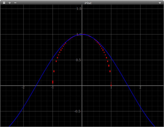
    plotWindow [ fnPlot cos
               , tracePlot [(x,y) | x<-[-1,-0.96..1]
                                  , y<-[0,0.01..1]
                                  , abs (x^2 + y^2 - 1) < 0.01 ]]
This gives such a plot window:
And that can with the mouse wheel be zoomed/browsed, like

The individual objects you want to plot can be evaluated in multiple threads, so
a single hard calculatation won't freeze the responsitivity of the whole window.
Invoke e.g. from ghci +RTS -N4 to benefit from this.
Plottable objects
Class
class Plottable p where Source
Methods
plot :: p -> DynamicPlottable Source
Simple function plots
fnPlot :: (forall m. Manifold m => ProxyVal (:-->) m Double -> ProxyVal (:-->) m Double) -> DynamicPlottable Source
Plot a continuous function in the usual way, taking arguments from the
x-Coordinate and results to the y one.
The signature looks more complicated than it is; think about it as requiring
a polymorphic Floating function. Any simple expression like
fnPlot (\x -> sin x / exp (x^2))
Under the hood this uses the category of continuous functions, :-->, to proove
that no details are omitted (like small high-frequency bumps). The flip side is that
this does not always work very efficiently, in fact it can easily become exponentially
slow for some parameters.
Make sure to run multithreaded, to prevent hanging your program this way. Also consider
limiting the memory: if you try to plot across singularities, the program may well
eat up all available resorces before failing. (But it will never “succeed” and
plot something wrong!)
In the future, we would like to switch to the category of piecewise continuously-differentiable functions. That wouldn't suffer from said problems, and should also generally be more efficient. (That category is not yet implemented in Haskell.)
paramPlot :: (forall m. Manifold m => ProxyVal (:-->) m Double -> (ProxyVal (:-->) m Double, ProxyVal (:-->) m Double)) -> DynamicPlottable Source
Plot a continuous, “parametric function”, i.e. mapping the real line to a path in ℝ².
continFnPlot :: (Double -> Double) -> DynamicPlottable Source
Plot an (assumed continuous) function in the usual way.
Since this uses functions of actual Double values, you have more liberty
of defining functions with range-pattern-matching etc., which is at the moment
not possible in the :--> category.
However, because Double can't really proove properties of a mathematical
function, aliasing and similar problems are not taken into account. So it only works
accurately when the function is locally linear on pixel scales (what most
other plot programs just assume silently). In case of singularities, the
naïve thing is done (extend as far as possible; vertical line at sign change),
which again is common enough though not really right.
We'd like to recommend using fnPlot whenever possible, which automatically adjusts
the resolution so the plot is guaranteed accurate (but it's not usable yet for
a lot of real applications).
tracePlot :: [(Double, Double)] -> DynamicPlottable Source
Plot a sequence of points (x,y). The appearance of the plot will be automatically
chosen to match resolution and point density: at low densities, each point will simply
get displayed on its own. When the density goes so high you couldn't distinguish
individual points anyway, we switch to a “trace view”, approximating
the probability density function around a “local mean path”, which is
rather more insightful (and much less obstructive/clunky) than a simple cloud of
independent points.
In principle, this should be able to handle vast amounts of data (so you can, say, directly plot an audio file); at the moment the implementation isn't efficient enough and will get slow for more than some 100000 data points.
View selection
xInterval :: (Double, Double) -> DynamicPlottable Source
When you “plot” xInterval / yInterval, it is ensured that the (initial) view encompasses
(at least) the specified range.
Note there is nothing special about these “flag” objects: any Plottable can request a
certain view, e.g. for a discrete point cloud it's obvious and a function defines at least
a y-range for a given x-range. Only use explicit range when necessary.
yInterval :: (Double, Double) -> DynamicPlottable Source
When you “plot” xInterval / yInterval, it is ensured that the (initial) view encompasses
(at least) the specified range.
Note there is nothing special about these “flag” objects: any Plottable can request a
certain view, e.g. for a discrete point cloud it's obvious and a function defines at least
a y-range for a given x-range. Only use explicit range when necessary.
Plot type
data DynamicPlottable Source