| Copyright | (c) Justus Sagemüller 2013-2015 |
|---|---|
| License | GPL v3 |
| Maintainer | (@) sagemueller $ geo.uni-koeln.de |
| Stability | experimental |
| Portability | requires GHC>6 extensions |
| Safe Haskell | None |
| Language | Haskell2010 |
Graphics.Dynamic.Plot.R2
Contents
Description
- plotWindow :: [DynamicPlottable] -> IO GraphWindowSpec
- class Plottable p where
- plot :: p -> DynamicPlottable
- fnPlot :: (forall m. Object (RWDiffable ℝ) m => AgentVal (-->) m ℝ -> AgentVal (-->) m ℝ) -> DynamicPlottable
- paramPlot :: (forall m. (WithField ℝ PseudoAffine m, SimpleSpace (Needle m)) => AgentVal (-->) m ℝ -> (AgentVal (-->) m ℝ, AgentVal (-->) m ℝ)) -> DynamicPlottable
- continFnPlot :: (Double -> Double) -> DynamicPlottable
- tracePlot :: [(Double, Double)] -> DynamicPlottable
- lineSegPlot :: [(Double, Double)] -> DynamicPlottable
- linregressionPlot :: forall x m y. (SimpleSpace m, Scalar m ~ ℝ, y ~ ℝ, x ~ ℝ) => (x -> m +> y) -> [(x, Shade' y)] -> (Shade' m -> DynamicPlottable -> DynamicPlottable -> DynamicPlottable) -> DynamicPlottable
- type PlainGraphicsR2 = Diagram B
- shapePlot :: PlainGraphicsR2 -> DynamicPlottable
- diagramPlot :: PlainGraphicsR2 -> DynamicPlottable
- plotLatest :: Plottable x => [x] -> DynamicPlottable
- tint :: Colour ℝ -> DynamicPlottable -> DynamicPlottable
- autoTint :: DynamicPlottable -> DynamicPlottable
- legendName :: String -> DynamicPlottable -> DynamicPlottable
- plotDelay :: NominalDiffTime -> DynamicPlottable -> DynamicPlottable
- xInterval :: (Double, Double) -> DynamicPlottable
- yInterval :: (Double, Double) -> DynamicPlottable
- forceXRange :: (Double, Double) -> DynamicPlottable
- forceYRange :: (Double, Double) -> DynamicPlottable
- newtype ViewXCenter = ViewXCenter {}
- newtype ViewYCenter = ViewYCenter {}
- newtype ViewWidth = ViewWidth {}
- newtype ViewHeight = ViewHeight {}
- newtype ViewXResolution = ViewXResolution {}
- newtype ViewYResolution = ViewYResolution {}
- dynamicAxes :: DynamicPlottable
- noDynamicAxes :: DynamicPlottable
- type DynamicPlottable = DynamicPlottable' RVar
- tweakPrerendered :: (PlainGraphicsR2 -> PlainGraphicsR2) -> DynamicPlottable -> DynamicPlottable
Interactive display
plotWindow :: [DynamicPlottable] -> IO GraphWindowSpec Source
Plot some plot objects to a new interactive GTK window. Useful for a quick preview of some unknown data or real-valued functions; things like selection of reasonable view range and colourisation are automatically chosen.
Example:
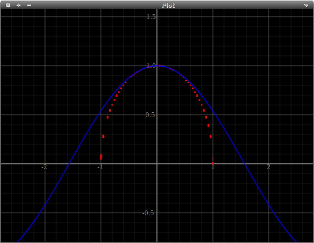
    plotWindow [ fnPlot cos
               , tracePlot [(x,y) | x<-[-1,-0.96..1]
                                  , y<-[0,0.01..1]
                                  , abs (x^2 + y^2 - 1) < 0.01 ]]
This gives such a plot window:
And that can with the mouse wheel be zoomed/browsed, like
The individual objects you want to plot can be evaluated in multiple threads, so
a single hard calculatation won't freeze the responsitivity of the whole window.
Invoke e.g. from ghci +RTS -N4 to benefit from this.
ATTENTION: the window may sometimes freeze, especially when displaying
complicated functions with fnPlot from ghci. This is apparently
a kind of deadlock problem with one of the C libraries that are invoked,
At the moment, we can recommend no better solution than to abort and restart ghci
(or what else you use – iHaskell kernel, process, ...) if this occurs.
Plottable objects
Class
class Plottable p where Source
Class for types that can be plotted in some canonical, “obvious”
way. If you want to display something and don't know about any specific caveats,
try just using plot!
Methods
plot :: p -> DynamicPlottable Source
Instances
| Plottable DynamicPlottable Source | |
| Plottable p => Plottable [p] Source | |
| Plottable p => Plottable (Maybe p) Source | |
| Plottable p => Plottable (Option p) Source | |
| Plottable (Shade' ℝ²) Source | |
| Plottable (Shade ℝ²) Source | |
| Plottable (ConvexSet ℝ²) Source | |
| Plottable p => Plottable (ViewHeight -> p) Source | |
| Plottable p => Plottable (ViewWidth -> p) Source | |
| Plottable p => Plottable (ViewYCenter -> p) Source | |
| Plottable p => Plottable (ViewXCenter -> p) Source | |
| Plottable (Shaded ℝ ℝ) Source | |
| Plottable (PointsWeb (ℝ, ℝ) (Colour ℝ)) Source | |
| Plottable (PointsWeb (ℝ, ℝ) (Shade (Colour ℝ))) Source | |
| Plottable (PointsWeb ℝ² (Colour ℝ)) Source | |
| Plottable (PointsWeb ℝ² (Shade (Colour ℝ))) Source | |
| Plottable (PointsWeb ℝ (Shade' ℝ)) Source |
Simple function plots
fnPlot :: (forall m. Object (RWDiffable ℝ) m => AgentVal (-->) m ℝ -> AgentVal (-->) m ℝ) -> DynamicPlottable Source
Plot a continuous function in the usual way, taking arguments from the
x-Coordinate and results to the y one.
The signature looks more complicated than it is; think about it as requiring
a polymorphic Floating function. Any simple expression like
fnPlot (\x -> sin x / cos (sqrt x))
Under the hood this uses the category of region-wise differentiable functions,
RWDiffable, to prove that no details are omitted (like small high-frequency
bumps). Note that this can become difficult for contrived cases like cos(1/sin x)
– while such functions will never come out with aliasing artifacts, they also
may not come out quickly at all. (But for well-behaved functions, using the
differentiable category actually tends to be more effective, because the algorithm
immediately sees when it can describe an almost-linear region with only a few line
segments.)
This function is equivalent to using plot on an RWDiffable arrow.
paramPlot :: (forall m. (WithField ℝ PseudoAffine m, SimpleSpace (Needle m)) => AgentVal (-->) m ℝ -> (AgentVal (-->) m ℝ, AgentVal (-->) m ℝ)) -> DynamicPlottable Source
Plot a continuous, “parametric function”, i.e. mapping the real line to a path in ℝ².
continFnPlot :: (Double -> Double) -> DynamicPlottable Source
Plot an (assumed continuous) function in the usual way.
Since this uses functions of actual Double values, you have more liberty
of defining functions with range-pattern-matching etc., which is at the moment
not possible in the :--> category.
However, because Double can't really prove properties of a mathematical
function, aliasing and similar problems are not taken into account. So it only works
accurately when the function is locally linear on pixel scales (what most
other plot programs just assume silently). In case of singularities, the
naïve thing is done (extend as far as possible; vertical line at sign change),
which again is common enough though not really right.
We'd like to recommend using fnPlot whenever possible, which automatically adjusts
the resolution so the plot is guaranteed accurate (but it's not usable yet for
a lot of real applications).
tracePlot :: [(Double, Double)] -> DynamicPlottable Source
Plot a sequence of points (x,y). The appearance of the plot will be automatically
chosen to match resolution and point density: at low densities, each point will simply
get displayed on its own. When the density goes so high you couldn't distinguish
individual points anyway, we switch to a “trace view”, approximating
the probability density function around a “local mean path”, which is
rather more insightful (and much less obstructive/clunky) than a simple cloud of
independent points.
In principle, this should be able to handle vast amounts of data (so you can, say, directly plot an audio file); at the moment the implementation isn't efficient enough and will get slow for more than some 100000 data points.
lineSegPlot :: [(Double, Double)] -> DynamicPlottable Source
Simply connect the points by straight line segments, in the given order.
Beware that this will always slow down the performance when the list is large;
there is no &201d; as in tracePlot.
linregressionPlot :: forall x m y. (SimpleSpace m, Scalar m ~ ℝ, y ~ ℝ, x ~ ℝ) => (x -> m +> y) -> [(x, Shade' y)] -> (Shade' m -> DynamicPlottable -> DynamicPlottable -> DynamicPlottable) -> DynamicPlottable Source
type PlainGraphicsR2 = Diagram B Source
Use plot to directly include any Diagram.
(All DynamicPlottable
is internally rendered to that type.)
The exact type may change in the future: we'll probably stay with diagrams,
but when document output is introduced the backend might become variable
or something else but Cairo.
shapePlot :: PlainGraphicsR2 -> DynamicPlottable Source
Use a generic diagram within a plot.
Like with the various specialised function plotters, this will get automatically
tinted to be distinguishable from other plot objects in the same window.
Use diagramPlot instead, if you want to view the diagram as-is.
diagramPlot :: PlainGraphicsR2 -> DynamicPlottable Source
Plot a generic Diagram.
Computation in progress
plotLatest :: Plottable x => [x] -> DynamicPlottable Source
Plot-object attributes
Colour
tint :: Colour ℝ -> DynamicPlottable -> DynamicPlottable Source
Colour this plot object in a fixed shade.
autoTint :: DynamicPlottable -> DynamicPlottable Source
Allow the object to be automatically assigned a colour that's otherwise unused in the plot. (This is the default for most plot objects.)
Legend captions
legendName :: String -> DynamicPlottable -> DynamicPlottable Source
Set the caption for this plot object that should appear in the plot legend.
Animation
plotDelay :: NominalDiffTime -> DynamicPlottable -> DynamicPlottable Source
Limit the refresh / frame rate for this plot object. Useful to slowly
study some sequence of plots with plotLatest, or to just reduce processor load.
Note: the argument will probably change to NominalDiffTime from the thyme library soon.
Viewport
View selection
xInterval :: (Double, Double) -> DynamicPlottable Source
When you “plot” xInterval / yInterval, it is ensured that the (initial) view encompasses
(at least) the specified range.
Note there is nothing special about these “flag” objects: any Plottable can request a
certain view, e.g. for a discrete point cloud it's obvious and a function defines at least
a y-range for a given x-range. Only use explicit range when necessary.
yInterval :: (Double, Double) -> DynamicPlottable Source
forceXRange :: (Double, Double) -> DynamicPlottable Source
Like xInterval, this only affects what range is plotted. However, it doesn't merely
request that a certain interval should be visible, but actually enforces particular
values for the left and right boundary. Nothing outside the range will be plotted
(unless there is another, contradicting forceXRange).
forceYRange :: (Double, Double) -> DynamicPlottable Source
View dependence
newtype ViewXCenter Source
ViewXCenter, ViewYResolution etc. can be used as arguments to some object
you plot, if its rendering is to depend explicitly on the screen's visible range.
You should not need to do that manually except for special applications (the
standard plot objects like fnPlot already take the range into account anyway)
– e.g. comparing with the linear regression of all visible points
from some sample with some function's tangent at the screen center.
plotWindow [fnPlot sin, plot $ \(ViewXCenter xc) x -> sin xc + (x-xc) * cos xc]

Constructors
| ViewXCenter | |
Fields | |
Instances
| Plottable p => Plottable (ViewXCenter -> p) Source |
newtype ViewYCenter Source
Constructors
| ViewYCenter | |
Fields | |
Instances
| Plottable p => Plottable (ViewYCenter -> p) Source |
Constructors
| ViewWidth | |
Fields | |
newtype ViewHeight Source
Constructors
| ViewHeight | |
Fields | |
Instances
| Plottable p => Plottable (ViewHeight -> p) Source |
newtype ViewXResolution Source
Constructors
| ViewXResolution | |
Fields | |
newtype ViewYResolution Source
Constructors
| ViewYResolution | |
Fields | |
Auxiliary plot objects
dynamicAxes :: DynamicPlottable Source
Coordinate axes with labels. For many plottable objects, these will be added
automatically, by default (unless inhibited with noDynamicAxes).
The plot type
type DynamicPlottable = DynamicPlottable' RVar Source